Window Functions and Parameterized SQL Queries

Practice with SQL window functions and parameterized queries from R using Olympics data.

After finishing the capstone project for the Learn SQL Basics for Data Science specialization on Coursera, I wanted to use the database I created to explore two other SQL topics: window functions and parameterized queries.

Database Setup

The capstone project provided two CSV files from which to create a normalized database of Olympic data.

My general process was to:

• Create a local PostgreSQL database.
• Run a script to create raw tables with empty integer ID columns.
• Copy the two provided CSV files into the raw tables with psql.
• Run another script that does the following:
  • Convert “NA” string data into SQL nulls.
  • Create and fill any tables without foreign keys.
  • Backfill the IDs into the raw table.
  • Use the IDs in the raw table to create tables requiring foreign keys.

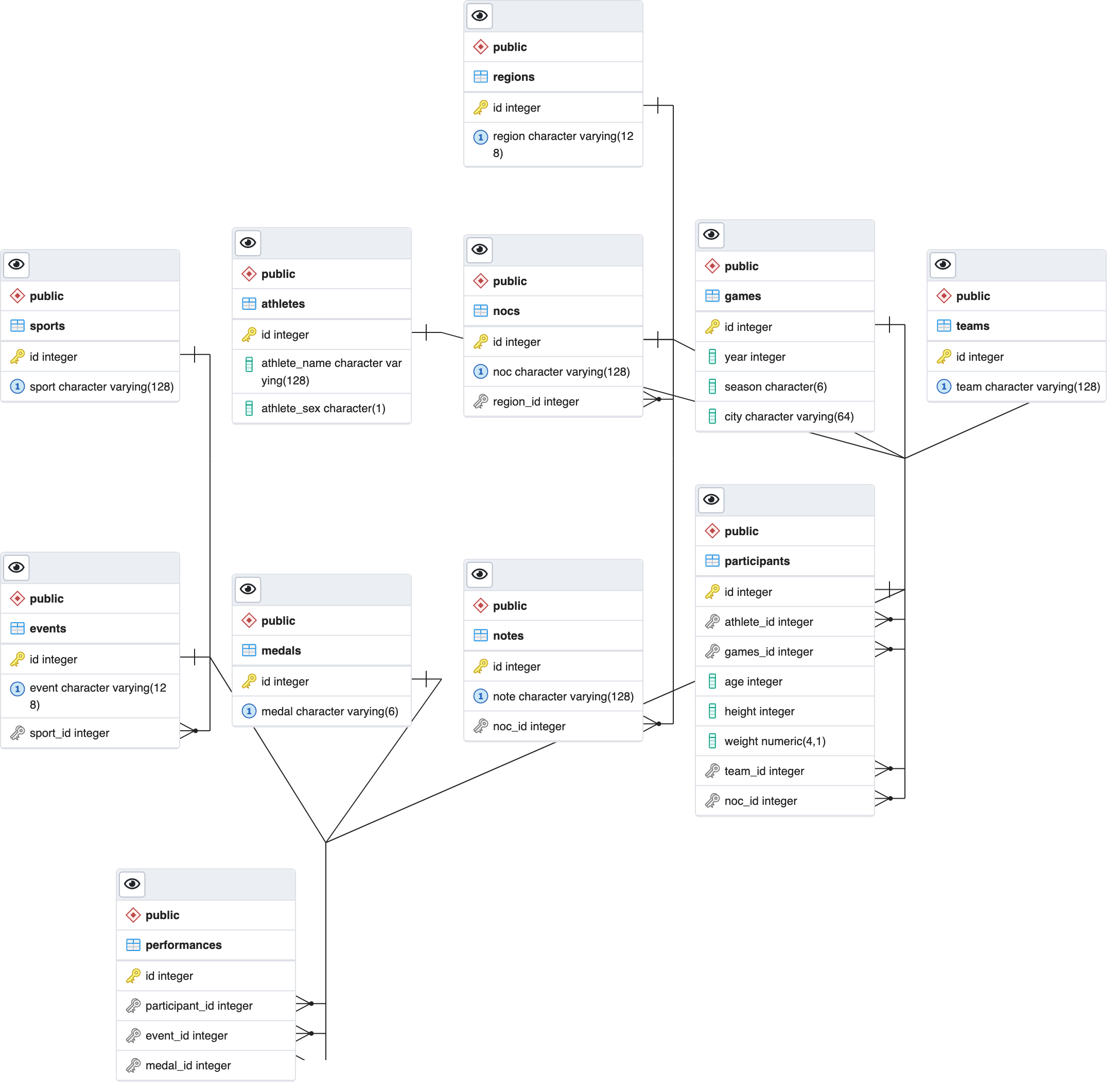
Here is the resulting ERD:

ERD of Olympic database

Defining a “Country”

One difficulty working with this data was trying to define a “country”. Given the long period of Olympic history, there’s no perfect definition of what constitutes a country since names change often. In this data, you’ll find columns noc (national organizing committee), region, team, and note that all contain some amount of country information.

Ultimately for this analysis, I’ve stuck with NOC as the best approximation of a country. Though you can see from the results below that a “region” like Germany has had four different NOCs, which means I’m effectively undercounting Germany’s Olympic performance over time by just looking at counts by NOC.

SELECT region, 
    COUNT(*) AS noc_count, 
    STRING_AGG(DISTINCT noc, ',') AS nocs
FROM nocs n
JOIN regions r
    ON n.region_id = r.id
GROUP BY region
ORDER BY noc_count DESC, region
LIMIT 5;

Table 1: 5 records

region	noc_count	nocs
Germany	4	FRG,GDR,GER,SAA
Czech Republic	3	BOH,CZE,TCH
Malaysia	3	MAL,MAS,NBO
Russia	3	EUN,RUS,URS
Serbia	3	SCG,SRB,YUG

Cumulative Medal Counts

This Coursera guided project offered a nice introduction to window functions, and so cumulative medal counts by NOC was a natural way to practice this set of functions.

In order to make the final plot clearer, I filtered the results by the top 10 all-time NOCs. To do so, I saved these 10 NOCs in a CTE and used them in a subquery.

WITH top_10_medals_by_noc AS (
    SELECT noc
    FROM performances pe
    JOIN participants pa
        ON pe.participant_id = pa.id 
    JOIN nocs n
        ON n.id = pa.noc_id
    WHERE medal_id IS NOT NULL
    GROUP BY noc
    ORDER BY COUNT(medal_id) DESC
    LIMIT 10
)

SELECT g.year, g.season, g.city, n.noc, 
    COUNT(pe.medal_id) AS medals,
    SUM(COUNT(pe.medal_id)) OVER (
        PARTITION BY noc
        ORDER BY year, season
        ROWS BETWEEN UNBOUNDED PRECEDING 
            AND CURRENT ROW) AS cum_medals
FROM performances pe
JOIN participants pa
    ON pe.participant_id = pa.id 
JOIN games g
    ON g.id = pa.games_id
JOIN nocs n
    ON n.id = pa.noc_id
WHERE noc IN (SELECT * FROM top_10_medals_by_noc)
GROUP BY g.year, g.season, g.city, n.noc
ORDER BY g.year;

I then output the result set to an R dataframe for a quick plot.

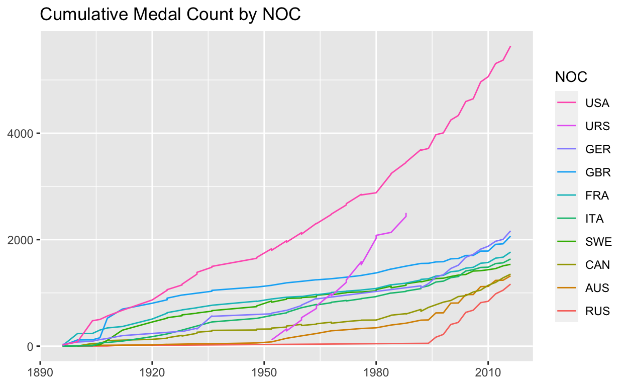
What’s most striking is the fast growth of the Soviet Union (URS), sudden stop, and then resumption of strong growth for Russia (RUS).

Parameterized SQL Queries with R

Although it wasn’t covered in the specialization, I wanted to get some practice running parameterized SQL queries with R following these safety guidelines. To simulate this, I saved to a folder a plot of performance statistics for each NOC.

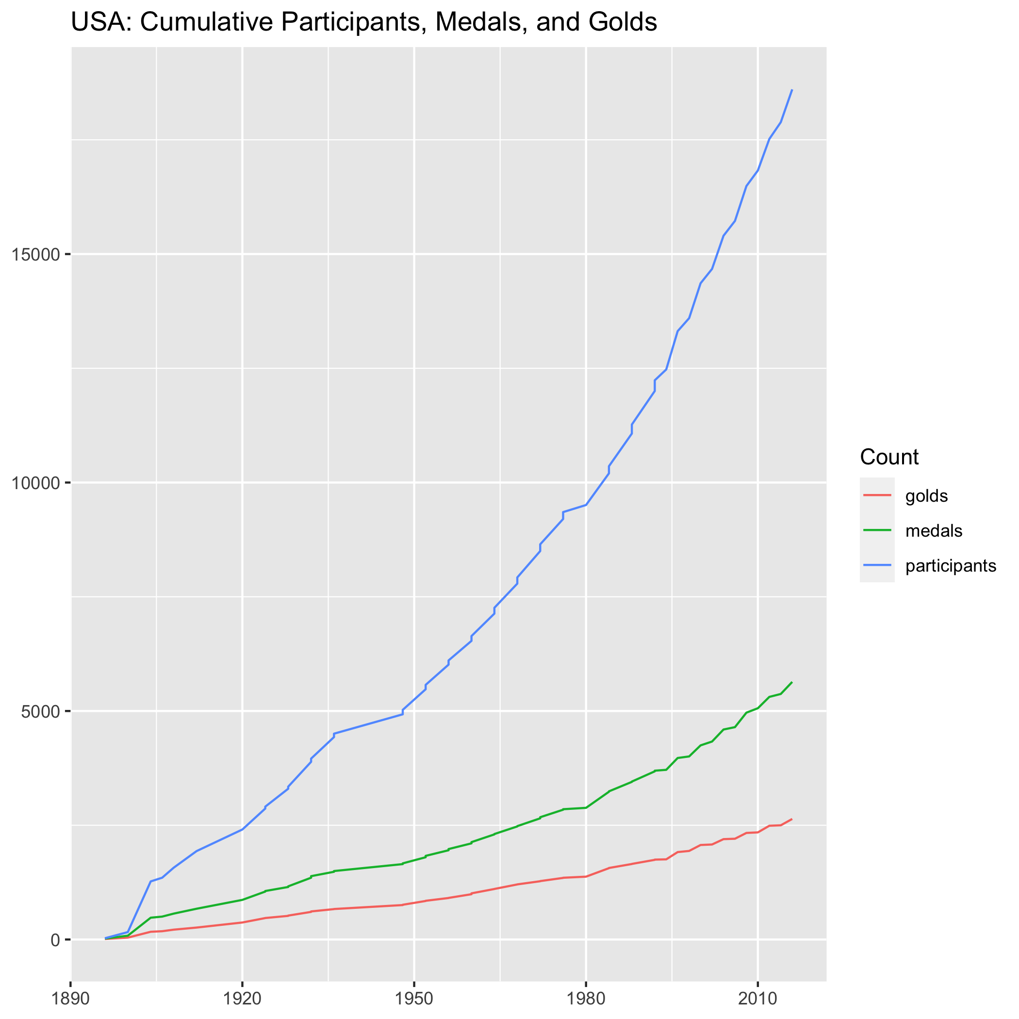
In addition to medals won, I also calculated the number of participants and gold medals won. To handle these additional metrics, I pivoted from wide to long format. PostgreSQL doesn’t have UNPIVOT, but you can do a lateral cross join.

I first got the parameterized query running, using $1 for the first (and only) parameter. Having the database safely execute it is then done by running through dbSendQuery(), dbBind(), dbFetch(), and dbClearResult() from the {DBI} package.

Once I got this working, I then looped over all 230 NOCs.

library(here)

# get vector of all nocs for loop
unique_nocs_df <- dbGetQuery(con, "SELECT noc FROM nocs")

# read parameterized query from file
query <- paste(readLines('noc_stats.sql'), collapse='\n')

if (!dir.exists("plots")) dir.create("plots")

for (i in unique_nocs_df$noc) {

    # send query with placeholder to db
    rs <- dbSendQuery(con, query)
    
    # bind parameters
    dbBind(rs, list(i))
    
    # fetch rows
    rows <- dbFetch(rs)
    
    # output plot
    mytitle <- paste0(i, ": Cumulative Participants, Medals, and Golds")
    temp_plot <- ggplot(rows, aes(x = year, y = value, 
                     fill = stat, color = stat)) +
        geom_line() +
        labs(title = mytitle, x = NULL, y = NULL, color = "Count")
    
    ggsave(temp_plot, file=here("plots", paste0(i,".png")))
    print(paste0("saving ", i))
    
    dbClearResult(rs)
}

dbDisconnect(con)

Here is the plot for the USA.

Plot of USA Olympic performance