Use R to structure and query database tables of Indian census data.
SQL
dbplyr
sf
PostGIS
rpostgis
Published
July 2, 2019
My recent blog posts have focused extensively on wrangling and visualizing data with R packages such as the {tidyverse}, {sf}, and {shiny}.
However, as the size of data grows beyond what can be stored in one’s local memory, along with a variety of other possible reasons, a relational database becomes more of a necessity. With this in mind, I have been exploring PostgreSQL, including how to access SQL databases without leaving the familiar confines of RStudio.
Previously, I wrangled together three decades of district-level Indian electricity and latrine access data. I used this dataset to:
highlight the wide district-level distribution behind any country-level statistic with a choropleth and histogram;
compare mapping styles such as bubble maps, dot density maps, and 3D choropleths;
create other visualizations that reveal the co-varying relationship between electricity and latrine access, such as a scatterplot and a bivariate choropleth.
In this post, I’ll demonstrate how I packaged this data into a PostGIS-enabled PostgreSQL database and how it can be queried from R. Specifically, this post covers:
Connecting to a SQL database from R
Writing data, including spatial data, to a remote database from R
Querying SQL databases from RStudio using SQL or {dplyr} syntax
In order to review how I created the R dataframes that I will write to the PostgreSQL database, please first examine this script here.
My previous dataframes were manipulated in such as way as to be prepared for their respective {shiny} applications. Thinking however of the most logical table structure for a database, I applied the following two steps. I divided country, state and district level data into separate tables. Moreover, I separated census data from spatial data.
Accordingly, I devised a database with three spatial tables (district and state shapes, plus another for the dot density map), three tables of census data (district, state and country-level), and one additional table of some useful state-identifying information such as state abbreviations, region, and union territory status. From these tables, I can use any combination of joins to create the data for any of the previous {shiny} apps.
Create a database
This blog among other resources suggest it is possible to create a new SQLite database directly from R. However, that does not appear to be as simple with PostgreSQL. As a rarer task, I’ll just create a locally-hosted database from pgAdmin, the GUI for PostgreSQL with a simple one line command.
CREATE DATABASE in_household;
Create a database connection
With the database initialized, I can start creating tables after establishing a connection. One can do this in R with the help of the {DBI} package.
The {DBI} package serves as a generic database interface for R. Packages like {RPostgres}, {RSQLite} or {RMySQL} then are implementations to forge connections between R and a particular database through the DBI interface.
For connecting to PostgreSQL from R, there are two possible implementation packages: {RPostgreSQL} and {RPostgres}. {Rpostgres} is newer and under more active development. According to this blog, it is also faster. However, when creating a connection via {RPostgres}, I had some trouble working with spatial data. This may be because I seem to be missing the correct driver. Nevertheless, there is also an {rpostgis} package with some handy functions that depends on the older {RPostgreSQL}. As speed won’t be a concern for me here, I’ll use the older {RPostgreSQL} implementation.
In the dbConnect() function from the {DBI} package, I specify PostgreSQL as the driver and give the database name. In many cases, here is where the user name and passwords would also be supplied.
Having connected to a database, I can now start writing data to it. I’ll start with the non-spatial data, demonstrating three methods.
The first writes a csv file through SQL code written in an R Markdown chunk, where SQL has been specified as the language engine.
The second directly writes an R dataframe through the DBI::dbWriteTable() function.
The third is a similar approach, but uses {dplyr}’s copy_to().
SQL’s CREATE TABLE and COPY statements
In an R Markdown document, I can change the language engine from the default of R to another language, such as SQL. I then just need to specify the existing connection made through the {DBI} package. The result below is the same as if entering the query directly in pgAdmin.
I do this in two stages. First I need a CREATE TABLE statement to initiate the table fields and associated constraints.
CREATETABLEIFNOTEXISTS states_abb_region_ut ( state varchar(90), -- state name, abb char(2) NOTNULL, -- state abbreviation region varchar(90) NOTNULL, -- state regionyeardateCHECK ((yearIN ('1991-01-01','2001-01-01','2011-01-01'))), -- state year (states change over time) ut_status booleanNOTNULL, -- is it a union territory?CONSTRAINT state_key PRIMARYKEY (state, year));
Then I use a COPY statement to import the data with a path to a local csv file.
Rather than first writing an R object to a CSV file, I can skip this intermediary step and, as shown below, directly write an R dataframe into a table in a remote database using the DBI::dbWriteTable() function.
# district_census is a dataframe in Rif (dbExistsTable(con, "district_census"))dbRemoveTable(con, "district_census")# Write the data frame to the databasedbWriteTable(con, name ="district_census", value = district_census, row.names =FALSE)
On exporting the data, SQL has made its best guess at the data type of each column. It recognized year as a date, and the count data as integers. It assigned non-numeric data as text and decimal numbers as real numbers.
If I want to alter the table, such as changing data types or assigning constraints like primary keys or NOT NULL requirements, I can do that through the dbExecute() function. In this case, the primary key for the “district_census” table is the unique combination of seven variables.
dbExecute(con,"ALTER TABLE district_census ALTER COLUMN geo_section TYPE char(8), ALTER COLUMN state TYPE varchar(90), ALTER COLUMN societal_section TYPE varchar(3), ALTER COLUMN demo_section TYPE char(5), ALTER COLUMN water_source TYPE varchar(90), ALTER COLUMN water_avail TYPE varchar(90), ALTER COLUMN district TYPE varchar(90);")
I could also use the {purrr} package to add constraints for columns requiring the same restrictions.
It shows that the primary key, checks on percentage columns, and not null columns have been successfully added to the table.
With {dplyr}
Similar to {DBI}’s dbWriteTable(), I can also directly write R dataframes to a remote database with {dplyr}.
{dplyr} is of course well-known as the {tidyverse}’s workhorse package for manipulation of data stored in local memory. However, with the help of {dbplyr}, it can also be used to manipulate data stored in remote databases.
{dplyr}’s copy_to() function, as explained in the {dbplyr} vignette, is a quick and dirty way to write a dataframe to a remote database. The command below adds the “state_census” dataframe to the database.
As with the dbWriteTable() method, I would need to subsequently alter any data types, keys and other constraints.
Because I had already written the necessary SQL import statements, I’ll use the first method to import the remaining table (country_census). This code can be found in the “write_tables_sql” folder.
Writing spatial data to a PostGIS-enabled PostgreSQL database
With the census data in place, I will now write the spatial data from R to the database. Doing so requires first installing the PostGIS extension. PostGIS is a spatial database extender for PostgreSQL. If you are familiar with R’s {sf} package, PostGIS will feel familiar– down to functions beginning with “ST_”.
One line of SQL code installs PostGIS.
CREATE EXTENSION postgis;
I can confirm the installation has been successful by checking the version number. (I’ll explain the dbGetQuery() function in a later section).
I can also confirm this through a function from the {rpostgis} package.
pgPostGIS(con)
PostGIS extension version 3.3.1 installed.
[1] TRUE
I’ll demonstrate two methods to write spatial data. The first writes an ESRI shapefile to a database through the command line. The second directly writes an {sf} object through the st_write() function.
Writing shapefiles via the command line
The first method of writing spatial data to a database does not involve R or RStudio at all. Instead it uses the command line. By opening a terminal window and navigating to the correct directory, I can write a shapefile with the following command. Note that this only works with the shapefile format and not other formats of spatial data.
shp2pgsql is a command line tool that comes with PostgreSQL for converting ESRI shapefiles into SQL suitable for insertion into a PostGIS-enabled PostgreSQL database.
Breaking down this command, note that:
-I adds a GiST index on the geometry column
-s 4326 specifies an SRID (Spatial Reference Identifier)
-W specifies the encoding
district_shapes.shp is the file name
district_shapes is the new table name
-d in_household is the database name
-U postgres is the default user
Directly writing spatial data with sf::st_write()
As in the first method shown for writing non-spatial data, the workflow above includes an intermediary step, in this case, the creation of an ESRI shapefile from the existing {sf} object. This may be useful in some cases, but ESRI shapefiles have certain limitations. For instance, field names greater than ten characters will be automatically abbreviated.
We should, however, be able to directly write an {sf} object to the database. I can do this with the st_write() function. Placing the st_write() function inside the purrr::walk() function provides for writing any number of spatial tables in a list or vector.
As shown below, I can confirm that the spatial data tables have been added with a function from the {rpostgis} package. I can also note that the file written as an ESRI shapefile has a geometry column named “geom”, whereas the objects written with st_write() hold their geometry in a column named “geometry”.
pgListGeom(con, geog =TRUE)
  schema_name               table_name geom_column geometry_type     type
1      public          district_shapes        geom  MULTIPOLYGON GEOMETRY
2      public electricity_latrine_dots    geometry      GEOMETRY GEOMETRY
3      public             state_shapes    geometry      GEOMETRY GEOMETRY
Querying SQL databases from R
Now that I have imported the requisite tables, I can begin querying the database from R. It is useful to first explore the database with a function like DBI::dbListTables() to see the names of the tables present.
Note that I did not explicitly create one table in the database, “spatial_ref_sys”. It gets created after installing the PostGIS extension.
Another useful {DBI} function is dbListFields() to examine the columns in a specific table by specifiying the connection and the table name.
dbListFields(con, "states_abb_region_ut")
[1] "state" "abb" "region" "year" "ut_status"
A similar {rpostgis} function gives a bit more information about the nature of the fields stored in any table.
dbTableInfo(con, "electricity_latrine_dots")
  column_name    data_type is_nullable character_maximum_length
1     sctl_sc         text         YES                       NA
2     dm_sctn         text         YES                       NA
3        year         date         YES                       NA
4     categry         text         YES                       NA
5           n      integer         YES                       NA
6      sum_hh      integer         YES                       NA
7    geometry USER-DEFINED         YES                       NA
Read an entire table into R
Having explored the contents of a database connection, I want to start pulling data from the database into R. To start, I can use the DBI::dbReadTable() function to import an entire remote table into R as a dataframe.
However, this is rarely optimal, especially if the tables are large. More often than not, you’ll only want a portion of a table stored in a database. In those situations, you want to query the database to retrieve some specified selection of a table.
That can be achieved in a number of different ways, including:
SQL code inside an R Markdown chunk with an SQL engine
SQL code inside the DBI::dbGetQuery() function
reference a dplyr::tbl() and query it with SQL
reference a dplyr::tbl() and query it with {dplyr} syntax
SQL inside an R Markdown chunk
The first option for querying an SQL database from R includes just writing SQL code inside an R Markdown chunk where the language engine has been changed to SQL, as demonstrated previously. The query below shows the ten states with the lowest rates of electricity access among rural ST households in 2011.
Using the output.var chunk option allows me to save the query output into a new dataframe. This however runs into the same problem as dbReadTable() for large datasets.
Another approach provides more query flexibility than dbReadTable() while staying within an R chunk to do the job. We can place any SQL query inside the dbGetQuery() function. Here we find the percentage of rural households among South Indian states having access to water within their household premises in 2011.
water_southern_2011 <-dbGetQuery(con,"SELECT s.state, num_total, num_within, ROUND(within::numeric, 2) AS water_within_home FROM state_census AS s LEFT JOIN states_abb_region_ut AS sabr ON s.state = sabr.state AND s.year = sabr.year WHERE region = 'Southern' AND s.year = '2011-01-01' AND societal_section = 'ALL' AND demo_section = 'Rural' AND water_source = 'All Sources' AND water_avail = 'Total' ORDER BY within DESC;")water_southern_2011
           state num_total num_within water_within_home
1         Kerala   4095674    2984553              0.73
2     Puducherry     95133      57764              0.61
3 Andhra Pradesh  14246309    4486906              0.31
4      Karnataka   7864196    2091969              0.27
5     Tamil Nadu   9563899    1625884              0.17
Not surprisingly, we can see that Kerala tops the list by a wide margin. Tamil Nadu’s rate is particularly poor.
The dbGetQuery() function returns a dataframe for the specified query. However, when dealing with large datasets, this may not always be the best form of output. Sometimes you may want a “lazier” approach.
class(water_southern_2011)
[1] "data.frame"
Reference a dplyr::tbl() and query it with SQL
With the addition of the {dbplyr} package, {dplyr} can be used to access data stored on a remote server. It is designed to be as lazy as possible in that it never pulls data into R unless explicitly requested.
For example, I can create a reference to a remote table with the tbl() function and execute a query wrapped inside the sql() function. Instead of a dataframe however, this returns a connection object.
Printing the object will show the data almost like a normal dataframe. However, it won’t return the number of observations (nrow() fails) because the data is not yet actually in R. The query below finds districts in 2011 with the largest raw difference between rates of household access to electricity and latrines.
largest_gap <-tbl(con, sql("SELECT state, district, ea, la, ABS(ea - la) AS gap FROM district_census WHERE year = '2011-01-01' AND societal_section = 'ALL' AND demo_section = 'Total' AND water_source = 'All Sources' AND water_avail = 'Total' ORDER BY gap DESC"))class(largest_gap)
{dbplyr} translates {dplyr} code to SQL before sending it to the database. We can actually see the SQL query generated from {dplyr} code using the show_query() function.
show_query(my_gap)
<SQL>
SELECT "state", "district", "ea", "la", ABS("ea" - "la") AS "gap"
FROM "district_census"
WHERE
  ("year" = '2011-01-01') AND
  ("societal_section" = 'ALL') AND
  ("demo_section" = 'Total') AND
  ("water_source" = 'All Sources') AND
  ("water_avail" = 'Total')
ORDER BY "gap" DESC
It’s not as readable as the original SQL code I wrote, but, on pasting it into pgAdmin, I can see that it works. The {dbplyr} vignette notes that it may not be the most natural SQL code for more complicated queries, but, if you don’t know any SQL, it’s a great substitute.
Use Cases
Thus far, the queries shown have been fairly simple. I now want to generate some more interesting queries.
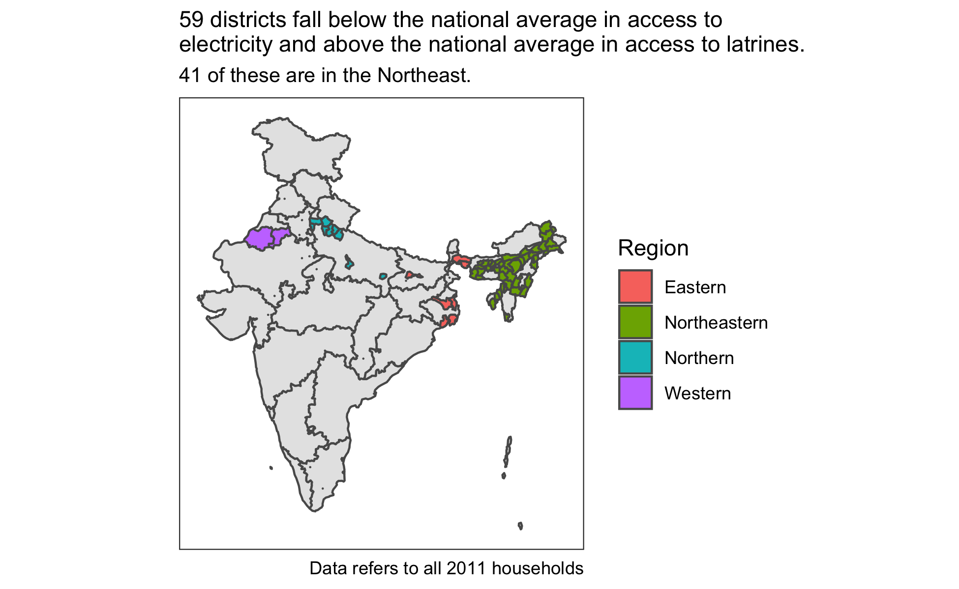
My project exploring how access to electricity covaries with access to latrines revealed a number of districts that fell below the national average in access to electricity, but above the national average in access to latrines. As this is an unusual combination, I want to query the database to find these districts.
Among all 2011 households, at the All-India level, 67% and 47% were the national averages for household access to electricity and latrines, respectively, as shown in the query below.
dbGetQuery(con,
            "SELECT ROUND(CAST(ea AS NUMERIC), 2) AS electricity,
                    ROUND(CAST(la AS NUMERIC), 2) AS latrines
            FROM country_census
            WHERE year = '2011-01-01' AND
                  societal_section = 'ALL' AND
                  demo_section = 'Total' AND
                  water_source = 'All Sources' AND
                  water_avail = 'Total'")
  electricity latrines
1        0.67     0.47
Next, with an SQL query in an R Markdown chunk with a SQL engine, I’ll save a view of all districts (matching the same year and other criteria) that fall below the national average in electricity access and above the national average in latrine access.
Then in the code below, I join two references to remote tables using the same {dplyr} syntax I would use to join two dataframes. Counting the districts by region reveals that 41 of these 59 regions fall in the Northeastern states.